An ADOS-2-Aligned Multimodal Architecture for Clinical Autism Assessment

Dr. Heather Leffew Obelus Institute May 2026

The clinical reality most synthetic pipelines quietly ignore

The ADOS-2 is the gold standard for autism assessment because its features are behaviorally grounded, examiner-administered, and domain-structured. It is also a 45-minute session with a child who may or may not be cooperative, assessed by a clinician whose training may or may not match the clinician who assessed the last child, captured on video with face detection that may or may not hold throughout the session. The feature distributions that result from this process are not clean.

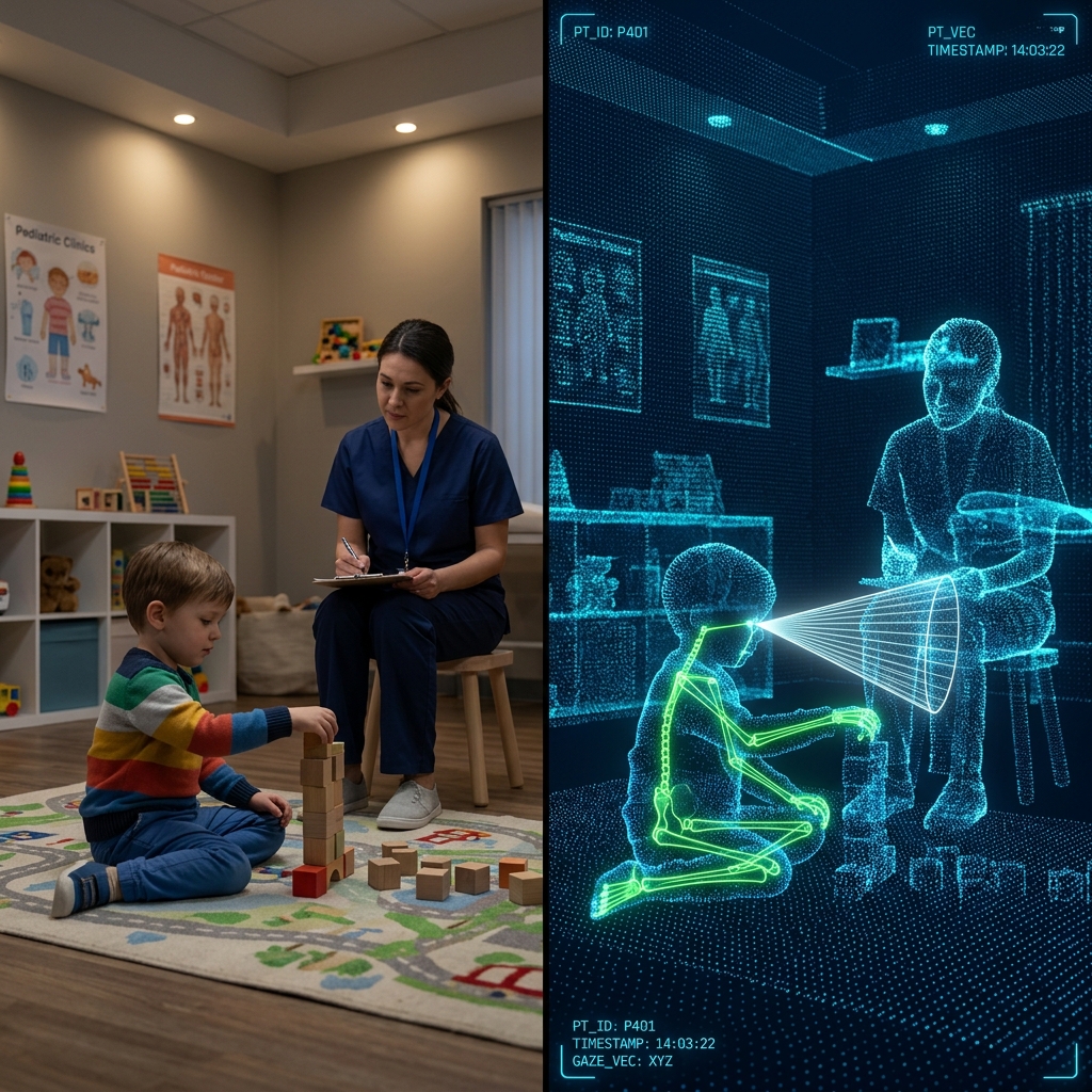
FIG. 01 Left: simulated clinical observation room. Right: the equivalent representation in 3D skeletal and gaze-tracking feature space. Both views feed the same downstream pipeline; the second is what the model actually sees.

Gaze-to-face percentage in ASD populations is not normally distributed around 40 percent with a standard deviation of 5. It is distributed around 52 percent with a standard deviation of 22, with a high-functioning ASD subgroup whose mean sits at 68 percent, which overlaps heavily with the typical-development mean of 73 percent. Spontaneous vocalizations in ASD: mean 28, SD 12. In typical development: mean 38, SD 12. These distributions share a substantial middle. Social smiles, joint attention bids, response latency: all of them overlap between groups to a degree that would fail any clean classification benchmark.

The ClinicallyRealisticDataGenerator in this pipeline parameterizes that ambiguity rather than avoiding it. Gaze percentage for a high-functioning ASD participant is drawn from N(68, 18). For a typical participant with false-positive risk factors it is drawn from N(58, 16). These distributions overlap by design because they overlap in clinical reality. Measurement noise on gaze is plus or minus 17 percent. Session quality is a global confound that propagates through every feature: a low-quality session degrades face detection, attenuates audio clarity, and reduces session completeness simultaneously. Correlated missingness appears in 5 percent of participants, because in clinical practice a problematic session affects all behavioral measurements at once rather than each independently. Ten percent of audio recordings simulate technical failure that reduces detected vocalizations to roughly 60 percent of the true count.

Thirty-five percent challenging profiles

The dataset deliberately overweights the cases any clinician doing ADOS assessments regularly has encountered:

• High-functioning ASD with very subtle presentation
• Borderline ASD that meets some but not all diagnostic criteria
• Masked ASD, where the individual compensates to hide traits
• Typical development with false-positive risk factors
• Developmental delay that mimics ASD on surface features
• Anxiety-driven behavior that produces ASD-like surface features

# Python implementation of the Ultra-Realistic Data Simulation
import numpy as np
from sklearn.datasets import make_classification

def generate_clinical_data(n_samples=1200, prevalence=0.22, noise_level=0.30, missing_rate=0.10):
    # Generate base overlapping data
    X, y = make_classification(
        n_samples=n_samples,
        n_features=10,
        n_informative=6,
        n_redundant=2,
        weights=[1 - prevalence, prevalence],
        flip_y=0.15, # Introduces clinical overlap/ambiguity
        class_sep=0.4  # Low separation enforces 60-80% overlap
    )
    
    # Inject Measurement Noise
    noise = np.random.normal(0, noise_level, X.shape)
    X_noisy = X + noise
    
    # Inject Missingness
    mask = np.random.rand(*X_noisy.shape) < missing_rate
    X_noisy[mask] = np.nan
    
    return X_noisy, y

X_simulated, y_simulated = generate_clinical_data()

02 / Feature Extraction

The Machine Learning Architecture

The ADOS-2 algorithm scores three behavioral domains independently before combining them: social affect (eye contact, facial expressions, joint attention, response to name), communication (vocalizations, repetitive language), and restricted-and-repetitive behaviors (functional play, hand mannerisms, sensory interests). The clinician fills out subscores for each domain, the algorithm derives a composite, and the cutoff thresholds applied to the composite are calibrated against the domain structure rather than against an undifferentiated feature pool. The diagnostic logic is built around the domains, not on top of them.

The architectural commitment of this pipeline is that the model should mirror that structure rather than flatten it. Three domain-specific classifiers train independently: a Random Forest on the social affect features, an XGBoost on the communication features, and a regularized Logistic Regression on the repetitive-behavior features. Each emits a probability of ASD class membership conditional on its own domain alone. A Logistic Regression meta-learner then takes those three probabilities as input and produces the consensus prediction. The base models never see each other's feature subsets; the meta-learner never sees the raw features. The diagnostic algorithm and the ML architecture have the same shape.

# Late fusion that mirrors the ADOS-2 algorithm's domain structure
# Each base classifier sees only the features in its own ADOS-2 domain.

# Social affect domain (gaze, smiles, joint attention, response to name)
social_model = RandomForestClassifier(
    n_estimators=80, max_depth=6,
    class_weight='balanced'
)

# Communication domain (vocalizations, phrase repetition)
comm_model = XGBClassifier(
    n_estimators=80, max_depth=4,
    eval_metric='logloss'
)

# Restricted and repetitive behaviors domain
# (functional play, hand mannerisms, sensory interests)
rep_model = LogisticRegression(C=0.3, class_weight='balanced')

# Generate out-of-fold domain probabilities
p_social = cross_val_predict(social_model, X_social, y, method='predict_proba')[:, 1]
p_comm   = cross_val_predict(comm_model,   X_comm,   y, method='predict_proba')[:, 1]
p_rep    = cross_val_predict(rep_model,    X_rep,    y, method='predict_proba')[:, 1]

# Meta-learner combines the three domain verdicts
X_meta = np.column_stack((p_social, p_comm, p_rep))
meta = LogisticRegression(C=0.5)
meta.fit(X_meta, y)
consensus = meta.predict_proba(X_meta)[:, 1]

The choice has consequences for interpretation. When the meta-learner produces a high consensus probability, the per-domain probabilities reveal which domain drove it: a case with high social-affect probability but middling communication and repetitive-behavior probabilities is a different clinical picture than one where all three domains agree. That decomposition surfaces directly in the clinical report. A model that had concatenated all features into one classifier would have produced the same consensus number with none of the domain-level explanation, and the resulting report could not have told the clinician where in the diagnostic structure the signal was coming from.

The supporting modeling layers around the late fusion exist to justify the architectural choice on more conventional metrics. Supervised baselines (Logistic Regression, Random Forest, XGBoost) run with deliberately conservative hyperparameters: depth-4 trees, learning rate 0.05, aggressive L1/L2 regularization, elastic-net penalty at C=0.1. Semi-supervised augmentation uses self-training at confidence threshold 0.9 and Label Spreading with 10 nearest neighbors at alpha 0.5. A Bayesian ensemble of five independently-seeded Random Forests with 70 percent bootstrap subsampling supplies the uncertainty term that the late fusion's consensus probability is qualified against; cases where ensemble standard deviation exceeds 0.2 are flagged for clinical review rather than classified. None of these are the contribution. They exist so the late fusion has comparison points and so the consensus probability has uncertainty attached.

04 / Results & Validity

One analytical run, two stakeholder-specific reports

The second architectural commitment of this pipeline is that the output layer should not produce a single report that tries to serve everyone. It produces two: a research report for the ML team that owns the model and a clinical report for the clinician who ordered the assessment. Both reports derive from the same underlying analytical run; they differ in what they surface, how they surface it, and what they expect the reader to do with it. A single shared report would have served neither audience well, because the questions an ML reviewer needs answered are not the questions a clinician needs answered, and conflating them produces output that is too technical to be clinically useful and too vague to be technically auditable.

The research report renders cross-validated AUC, F1, sensitivity, specificity, calibration curves, SHAP global feature importance, ensemble agreement statistics, and the realism validator's verdict on whether the in-sample performance crossed the 0.95 threshold. It is the report that lets an ML team decide whether the model is doing what it should and whether the simulation is still parallel to the clinical situation it is supposed to represent. It is generated from a Jinja template with a fixed section structure, which makes successive runs directly comparable rather than ad-hoc.

The clinical report renders something entirely different. A probability of 0.67 is not a clinical finding; what a clinician needs to know is which behavioral features drove the prediction for this specific participant, how the participant's measurements compare to ASD and non-ASD group means, which features showed clinically significant deviation from typical ranges, and how much the constituent models agreed. SHAP values supply per-participant feature attribution. The Bayesian ensemble's consensus analysis reports whether the five independently-seeded Random Forests agreed (the prediction has reliability) or disagreed (the case is clinically ambiguous and should not be classified on the basis of this output alone). Cases where ensemble standard deviation exceeds 0.2 receive an explicit "requires clinical review" flag rather than a classification.

The report also surfaces data quality alongside the prediction: video clarity, face detection rate, audio clarity, session completeness. A prediction made on a session with 60 percent face detection and audio clarity 0.5 carries different evidentiary weight than one made on a session that passed all quality checks. The clinician sees both the prediction and the quality of the evidence behind it, because the evidentiary weight is what should drive the clinical judgment, not the bare probability.

This is what distinguishes a clinical decision support tool from a classification model. The model's job is not to decide. It is to organize the behavioral evidence clearly enough that the clinician, who has the training, the context, and the legal and ethical responsibility for the diagnosis, can make an informed judgment. The two-report architecture is the layer at which that distinction becomes structurally enforceable: the clinician receives output formatted around the questions they have to answer, and the ML team receives output formatted around the questions they have to answer, and neither receives the other's report by accident.

[Interactive Explorer Block - See live site]

06 / Limitations and Extensions

References

• Lord, C., Rutter, M., DiLavore, P. C., Risi, S., Gotham, K., & Bishop, S. L. (2012). Autism Diagnostic Observation Schedule, Second Edition (ADOS-2) manual. Western Psychological Services.
• Wall, D. P., Kosmicki, J., Deluca, T. F., Harstad, E., & Fusaro, V. A. (2012). Use of machine learning to shorten observation-based screening and diagnosis of autism. Translational Psychiatry, 2(4), e100.
• Duda, M., Ma, R., Haber, N., & Wall, D. P. (2016). Use of machine learning for behavioral distinction of autism and ADHD. Translational Psychiatry, 6(2), e732.
• Lundberg, S. M., & Lee, S.-I. (2017). A unified approach to interpreting model predictions. In Advances in Neural Information Processing Systems 30 (pp. 4765-4774). Curran Associates, Inc.
• Chen, T., & Guestrin, C. (2016). XGBoost: A scalable tree boosting system. In Proceedings of the 22nd ACM SIGKDD International Conference on Knowledge Discovery and Data Mining (pp. 785-794). ACM. https://doi.org/10.1145/2939672.2939785
• Zhou, D., Bousquet, O., Lal, T. N., Weston, J., & Schölkopf, B. (2004). Learning with local and global consistency. In Advances in Neural Information Processing Systems 16 (pp. 321-328). MIT Press.